The world comprises of data, many data. Data is mostly in the form of documents, music, videos, pictures, and many more. Apart from us, the people, data is generated from many other resources like mobiles, tablets, computers, and other devices. Traditionally, humans have analyzed data and adapted systems to change in data patterns. However, the volume of data surpasses the ability for humans to make sense of it and manually write those rules.
Machine Learning brings the promise of deriving meaning from all of the data; it is an automated system that can learn from data and also the change in data to a shifting landscape. Machine learning is rapidly becoming an expected feature, and every company is pivoting to use it in their products in some way.
What is Machine Learning? [Definition]
Machine Learning can be brought down to five words:

Using data is referred to as training and answering questions refers to as making predictions or inference. Training refers to using our data to inform the creation and fine-tuning of the predictive model. The predictive model can be used up to serve up predictions on previously unseen data and answer those questions. The model can be improved over time as more data gathers, and new models can also be deployed.

The value of ML is beginning to show itself; things like tagging objects and people inside photos are machine learning at play. In video applications like YouTube, recommending the next video to watch is also powered by machine learning. The most used Google search engine has many machine learning systems at its core, from understanding the text of your query to adjusting the results based on your interests. Today, machine learning applications are already quite wide-ranging, including image recognition, fraud detection, and recommendation systems. Machine learning is used to make human tasks better, faster, and more comfortable than before. The day is not far when we would expect our technology to be personalized, insightful, and self-correcting.
How Does Machine Learning Work?
Machine learning under the hood is a 7 step model that comprises of :
- Gathering Data
- Data Preparation
- Choosing a model
- Training
- Evaluation
- Hyperparameter Tuning
- Prediction
Let us discuss now the workflow of ML with the help of an example:
In this example, we create a system that answers the question of whether the given drink is wine or beer.

This system builds to answer the question is called a model, and is created via a process of training. Machine learning requires us to build an accurate model that mostly answers our questions correctly. We need to collect the data to train the model, which is the first step in the process.
1. Gathering Data
The data is collected from the glasses of wine and beer. There are many aspects that we could collect data, everything from the amount of foam to the shape of the glass. In this example, we pick the color as the wavelength of light and the alcohol content as the percentage and refer to them as features. The first step involves us to buy a bunch of different drinks from our grocery store and also get some equipment to do our measurements a spectrometer to measure our color and a hydrometer to measure the alcohol content.
The step of gathering data is essential because the quality or quantity of the data gathered determines the quality of the predictive model. Collecting the color and alcohol content of each drink yields a table of color, alcohol content, and whether it is beer or wine, which is our training data.
2. Data Preparation
The step requires to load data into a suitable place and prepare it for our machine learning training.
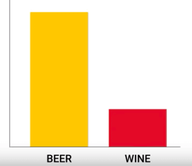
We put our data and then randomize the ordering because we don’t want the system to learn that is not part of determining whether a drink is a beer or wine. The system must have the ability to determine the drink, whether it is beer or wine, irrespective of the sequence. Pertinent visualizations can also be performed at this stage to see if there exists any relevant relationship between different variables and also see if there are any data imbalances. If we collect more data points for beer than wine, then the trained model heavily biased towards guessing that virtually everything that it sees is beer since it would be right most of the time. However, in the real world, the model might come across an equal amount of wine and beer, and so it would be guessing the wrong beer half of the time.
We also split the data into two parts, the first part used in training the model is the dataset, and the second part is used for evaluating the trained model’s performance. Evaluation of the model’s performance is required as we won’t use the same data from which the model was trained since it would be able to memorize the questions. Data collected sometimes needs manipulation like duplication, normalization, error correction, and others. The data preparation step adjusts data accordingly.
Machine Learning A-Z™: Python & R in Data Science [2024]
3. Choosing a Data Model
There are several models that researchers and data scientists have created over the years. Some are well suited for image data and others for sequences such as text or music, some for numerical data. In our case, we use a small linear model since we have two features- color and alcohol.

4. Training
Training is also the bulk of the machine learning process. This step uses data to incrementally improve the model’s ability to predict whether a given drink is wine or beer. The formula for a straight line is

Where x denotes the input, m is the slope of the line, b is the y-intercept, and y is the value of line at that position x. Slope m and y-intercept b are the only values available to adjust or train. There exists no other way to affect the position of the line since the only variables are x, the input, and y, the output. In machine learning, there exist several m’s since there may be many features. A matrix known as the weight matrix w is constructed from these values.

Similarly, for b, we arrange them together and call them biases. The training involves initializing some random values for w and b and attempting to predict the outputs for those values. Although it performs poorly at first, the model’s prediction can be compared with the output that it should have produced and adjust the values in w and b, so that has a more accurate prediction next time. So this process repeats. Each iteration or cycle of updating weights and biases is called one training step.
5. Evaluation
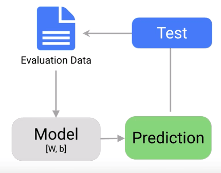
Once the training completes, it is time to evaluate the model to see if it is competent and well trained. Evaluation allows us to test our model against data that has never used for training. The metric allows us to see how the model might perform against data that it has not yet seen. Evaluation is meant to represent how the model might perform in the real world.
6. Hyperparameter Tunning
After tunning, we perform tuning to check if there is further room for improvement in the training; this is done by tuning some of our parameters. Listed below are the examples of parameter tuning that can be performed:
How many times trained set runs during training: We can show data multiple times, and by doing this, we potentially lead to higher accuracies.
Learning Rate: The learning rate defines how far the line shifts during each step based on the information from the previous training step. For complex models, initial conditions can play a significant role as well as determining the outcome of training. Differences are seen depending upon whether a model starts of training with values initialized at zero versus some distribution of the values.
During this phase of training, there are many considerations, and one must specify and define what makes a useful model for you; otherwise, we might find ourselves tweaking parameters for a long time.
These parameters are called hyperparameters.
7. Prediction or Inference

We can finally test the model to predict if a given drink is wine or beer, given its’ color or alcohol percentage. Machine learning enables us to differentiate between wine and beer using the model rather than human judgment and standard rules.
Types of Machine Learning

1. Supervised Learning
The method of learning involves overseeing or directing a particular activity and make sure it is done correctly. It is a method in which we teach the machine using labeled data.
It solves two kinds of problems:
Regression: It is a predictive analysis used to predict continuous variables. E.g., predicting the price of the stock.
Classification: It involves predicting a label or a class. E.g., classifying emails as spam or not spam.
2. Unsupervised Learning
In this type of learning, the machine is trained on unlabeled data without any guidance. It discovers hidden patterns and trends in the data.
It solves two kinds of problem:
Association: It involves discovering patterns in data, finding co-occurrences, and more.
Clustering and Anomaly Detection: Clustering involves targeted marketing, whereas anomaly detection tracks unusual activities. Eg. Credit card frauds.
Check here: Difference between Supervised and Unsupervised Learning
3. Reinforcement Learning
In this learning, an agent interacts with the environment by producing actions and discover errors and rewards. E.g. In the beginning, an untrained robot knows nothing about the surroundings in which is it exists. So after performing specific actions, it finds more about its surroundings. Robot here is known as the agent, and the surroundings are the environment, so for each action, it takes it can receive reward or punishment.
Applications of Machine Learning
1. Virtual Assistants
Google Assistants, Alexa, Cortana, Siri, and many other google assistants like them improve our lives in a significant way. They work by recording what we say and then send it to the server, which is the cloud. The code then is decoded with the help of machine learning, and neural network, and then output is provided. The system strives to work without WiFi, as it cannot contact the server.
2. Traffic Predictions
Maps predict whether the traffic is clear, slow-moving, or heavily-congested based on two measures:

The average time taken on specific days at specific times at that route.
Real-time location data of vehicles from google maps applications and sensors.
3. Social Media Personalization
All of us have noticed that if we search online about some products that we are planning to buy, we end up with recommendations and advertisements about the product on other social websites and applications like Facebook and Instagram. The machine learning algorithm works behind recommending the products.
4. Email-Spam Filtering
The mails are analyzed and segregated as spam or not spam through the spam filters. It works by analyzing the collection of data and searching for keywords such as “lottery” or “winner” in the mails.
Spam filters are of following types:
- Content Filters
- Header Filters
- General Blacklist Filters
- Rule-Based Filters
- Permission Filters
- Challenge-Response Filters
5. Assistive Medical Technology
With the help of machine learning, medical technology has innovated to diagnose diseases. It allows analyzing 2D CT scans and comes up with 3D models that predict where exactly there are lesions in the brain. It works equally well for brain tumors and stroke lesions. It also applications in fetal imaging and cardiac analysis.
Salary for Machine Learning Engineer
|
1. Entry Level
|
|
2. Mid Level
|
|
3. Senior Level
|


Source: Payscale
Summary
Machine learning is becoming the trendy field of the century. Machine learning vs Artificial Intelligence is the talk of the town theses days since they both are used interchangeably, ML is merely the study of training a system to improve upon a set task that given progressively whereas AI is the development of machines to be able to behave and perform task like human brains.
ML has become a pivot feature that organizations want to add any of there products. It drives the idea of automation and making tasks easier for humans. It is gaining popularity and increasing the list of the area where it is used like in electronic devices, smart homes, agriculture, health, and many more. Machine learning is used in our daily lives in some or the other way. Do you use machine learning throughout the day? And is it helpful to you? How? Also, let us know the machine learning techniques that you prefer for development?
Let us know in the comments below!
People are also reading:
- Machine Learning Certification
- Machine Learning Books
- Machine learning Interview Questions
- What is Machine Learning?
- How to become a Machine Learning Engineer
- Types of Machine Learning
- Decision Tree in Machine Learning
- Machine Learning Algorithm
- Difference between Data Science vs Machine Learning
- Difference between Machine Learning and Deep Learning
