What is the Naive Bayes Algorithm?
The naive Bayes model, irrespective of the strong assumptions that it makes, is often used in practice, because of its simplicity and the small number classification of parameters required. The model is generally used for classification — deciding, based on the values of the evidence variables for a given instance, the class to which the instance is most likely to belong.
A Naive Bayes Classifier algorithm based on Bayes theorem, which offers an insight that it is possible to adjust the probability of an event as new data introduces. It is a probabilistic algorithm which means it calculates the probability of each tag for a given text, and then the output tag with the highest one. The algorithm is not a single one but a collection of different machine learning algorithms that use statistical independence, which is easy to write and run more efficiently than complex Bayes algorithms.
Working of Naive Bayes: Example
Classification
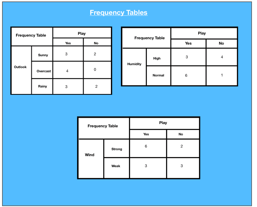
Suppose we have the dataset in which we have the outlook, the humidity and we need to find whether we should play or not on that day. The outlook could be a sunny overcast or rainy and the humidity is high or normal. The wind is categorized into two feeders which are weak winds and strong winds.
Dataset
| Day | Outlook | Humidity | Wind | Play |
| D1 | Sunny | High | Weak | No |
| D2 | Sunny | High | Strong | No |
| D3 | Overcast | High | Weak | Yes |
| D4 | Rain | High | Weak | Yes |
| D5 | Rain | Normal | Weak | Yes |
| D6 | Rain | Normal | Strong | No |
| D7 | Overcast | Normal | Strong | Yes |
| D8 | Sunny | High | Weak | No |
| D9 | Sunny | Normal | Weak | Yes |
| D10 | Rain | Normal | Weak | Yes |
| D11 | Sunny | Normal | Strong | Yes |
| D12 | Overcast | High | Strong | Yes |
| D13 | Overcast | Normal | Weak | Yes |
| D14 | Rain | High | Strong | No |
Frequency tables for each attribute of the data set are given as:
The following are the Likelihood tables generated for each frequency table:
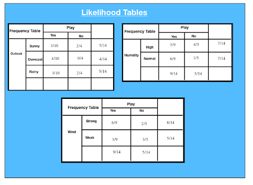
P(x|c) = P(Sunny|Yes) = 3/10 = 0.3
P(x) = P(Sunny) = 5/14 = 0.36
P(c) = P(Yes) = 10/14 = 0.71
Attribute: Outlook: Sunny
Likelihood of “Yes” given sunny is:
P(c|x) = P(Yes|Sunny) = P(Sunny|Yes) * P(Yes) | P(Sunny)
= 0.3 x 0.71/ 0.36 = 0.591
Likelihood of “No” given sunny is:
P(c|x) = P(No|Sunny) = P(Sunny|No) * P(No) | P(Sunny)
= 0.4 x 0.36 / 0.36 = 0.40
Attribute: Humidity: High
Likelihood of “Yes” given high humidity is:
P(c|x) = P(Yes|Humidity) = P(Humidity|Yes) * P(Yes) | P(High)
= 0.33 x 0.6 / 0.36 = 0.42
Likelihood of “No” given high humidity is:
P(c|x) = P(No|High) = P(High|No) * P(No) | P(High).
= 0.8 x 0.36 / 0.5 = 0.58
Attribute: Wind: Weak
Likelihood of “Yes” given weak wind is:
P(c|x) = P(Yes|Humidity) = P(Humidity|Yes) * P(Yes) | P(High)
= 0.67 x 0.64 / 0.57 = 0.75
Likelihood of “No” given weak wind is:
P(c|x) = P(No|High) = P(High|No) * P(No) | P(High)
= 0.4 x 0.36/ 0.57 = 0.25
Suppose we have a day with the following values:
Outlook: Rain
Humidity: High
Wind: Weak
Play:?
Likelihood of ‘No’ on that day.
P(Outlook= Rain|No) * P(Humidity=High|No) * P(Wind = Weak|No) * P(No)
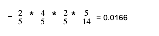
P(Yes)= 0.0199/ (0.0199 + 0.0166) = 0.55
P(No) = 0.0166 / (0.0199 + 0.0166)= 0.45
Thus, the model predicts that there is a 55% chance that there would be a game tomorrow.
Data Science & Machine Learning: Naive Bayes in Python
Steps involve Naive Bayes Algorithm
EXAMPLE: PIMA DIABETIC TEST
The problem comprises 768 observations of medical details of the patients’ records describes instantaneous measurement is taken from the patients such as they age, the number of times pregnant, blood workgroup. All the attributes are numeric and units vary from attribute to attribute. Each record has a class value that indicates whether the patients suffered on the set of diabetes within five years. The whole process can be brought down to five steps:
Step 1: Handling Data
Data is loaded from the CSV File and spread into training and tested assets.
Step 2: Summarizing the Data
Summarise the properties in the training data set to calculate the probabilities and make predictions.
Step 3: Making a Prediction
A particular prediction is made using a summarise of the data set to make a single prediction.
Step 4: Making all the Predictions
Generate prediction given a test data set and a summarise data set.
Step 5: Evaluate Accuracy
Accuracy of the prediction model for the test data set as a percentage correct out of them all the predictions made.
Step 6: Tying all Together
Finally, we tie to all steps together and form our own model of Naive Bayes Classifier.
Code
import csv
import random
import math
import numpy as np

def load_csv(filename):
 """
 :param filename: name of csv file
 :return: data set as a 2 dimensional list where each row in a list
 """
 lines = csv.reader(open(filename, 'r'))
 dataset = list(lines)
 for i in range(len(dataset)):
 dataset[i] = [float(x) for x in dataset[I]]
 return dataset
 # data = load_csv('pima-indians-diabetes.data.csv')
 # print(data)

def split_dataset(dataset, ratio):
 """
 split dataset into training and testing
 :param dataset: Two dimensional list
 :param ratio: Percentage of data to go into the training set
 :return: Training set and testing set
 """
 size_of_training_set = int(len(dataset) * ratio)
 train_set = []
 test_set = list(dataset)
 while len(train_set) < size_of_training_set:
 index = random.randrange(len(test_set))
 train_set.append(test_set.pop(index))
 return [train_set, test_set]

# training_set, testing_set = split_dataset(data, 0.67)
# print(training_set)
# print(testing_set)

def separate_by_label(dataset):
 """
 :param dataset: two dimensional list of data values
 :return: dictionary where labels are keys and
 values are the data points with that label
 """
 separated = {}
 for x in range(len(dataset)):
 row = dataset[x]
 if row[-1] not in separated:
 separated[row[-1]] = []
 separated[row[-1]].append(row)

return separated

# separated = separate_by_label(data)
# print(separated)
# print(separated[1])
# print(separated[0])

def calc_mean(last):

 return sum(lst) / float(len(last))

def calc_standard_deviation(last):
 avg = calc_mean(last)
 variance = sum([pow(x - avg, 2) for x in lst]) / float(len(lst) - 1)
 return math.sqrt(variance)

# numbers = [1, 2, 3, 4, 5]
# print(calc_mean(numbers))
# print(calc_standard_deviation(numbers))

def summarize_data(last):

 """
 Calculate the mean and standard deviation for each attribute
 :param lst: list
 :return: list with mean and standard deviation for each attribute
 """

 summaries = [(calc_mean(attribute), calc_standard_deviation(attribute))
 for attribute in zip(*lst)]
 del summaries[-1]

 return summaries

# summarize_me = [[1, 20, 0], [2, 21, 1], [3, 22, 0]]
# print(summarize_data(summarize_me))

def summarize_by_label(data):

 """
 Method to summarize the attributes for each label
 :param data:
 :return: dict label: [(atr mean, atr stdv), (atr mean, atr stdv)....]
 """
 separated_data = separate_by_label(data)
 summaries = {}
 for label, instances in separated_data.items():
 summaries[label] = summarize_data(instances)
 return summaries

# fake_data = [[1, 20, 1], [2, 21, 0], [3, 22, 1], [4,22,0]]
# fake_summary = summarize_by_label(fake_data)

def calc_probability(x, mean, standard_deviation):
 """
 :param x: value
 :param mean: average
 :param standard_deviation: standard deviation
 :return: probability of that value given a normal distribution
 """
 # e ^ -(y - mean)^2 / (2 * (standard deviation)^2)
 exponent = math.exp(-(math.pow(x - mean, 2) / (2 * math.pow(standard_deviation, 2))))
 # ( 1 / sqrt(2π) ^ exponent
 return (1 / (math.sqrt(2 * math.pi) * standard_deviation)) * exponent

# x = 57
# mean = 50
# stand_dev = 5
# print(calc_probability(x, mean, stand_dev))

def calc_label_probabilities(summaries, input_vector):
 """
 the probability of a given data instance is calculated by multiplying together
 the attribute probabilities for each class. The result is a map of class values
 to probabilities.
 :param summaries:
 :param input_vector:
 :return: dict
 """
 probabilities = {}
 for label, label_summaries in summaries.items():
 probabilities[label] = 1
 for i in range(len(label_summaries)):
 mean, standard_dev = label_summaries[I]
 x = input_vector[I]
 probabilities[label] *= calc_probability(x, mean, standard_dev)

return probabilities

# fake_input_vec = [1.1, 2.3]
# fake_probabilities = calc_label_probabilities(fake_summary, fake_input_vec)
# print(fake_probabilities)

def predict(summaries, input_vector):

 """
 Calculate the probability of a data instance belonging
 to each label. We look for the largest probability and return
 the associated class.
 :param summaries:
 :param input_vector:
 :return:
 """
 probabilities = calc_label_probabilities(summaries, input_vector)
 best_label, best_prob = None, -1
 for label, probability in probabilities.items():
 if best_label is None or probability > best_prob:
 best_prob = probability
 best_label = label
 return best_label

# summaries = {'A': [(1, 0.5)], 'B': [(20, 5.0)]}
# inputVector = 1.1
# print(predict(summaries, inputVector))

def get_predictions(summaries, test_set):

 """
 Make predictions for each data instance in our
 test dataset
 """
 predictions = []
 for i in range(len(test_set)):
 result = predict(summaries, test_set[i])
 predictions.append(result)

 return predictions

# summaries = {'A': [(1, 0.5)], 'B': [(20, 5.0)]}
# testSet = [1.1, 19.1]
# predictions = get_predictions(summaries, testSet)
# print(predictions)

def get_accuracy(test_set, predictions):

 """
 Compare predictions to class labels in the test dataset
 and get our classification accuracy
 """
 correct = 0
 for i in range(len(test_set)):
 if test_set[i][-1] == predictions[i]:
 correct += 1

 return (correct / float(len(test_set))) * 100

# fake_testSet = [[1, 1, 1, 'a'], [2, 2, 2, 'a'], [3, 3, 3, 'b']]
# fake_predictions = ['a', 'a', 'a']
# fake_accuracy = get_accuracy(fake_testSet, fake_predictions)
# print(fake_accuracy)

def main(filename, split_ratio):

 data = load_csv(filename)
 training_set, testing_set = split_dataset(data, split_ratio)
 print("Size of Training Set: ", len(training_set))
 print("Size of Testing Set: ", len(testing_set))

 # create model
 summaries = summarize_by_label(training_set)

 # test mode
 predictions = get_predictions(summaries, testing_set)
 accuracy = get_accuracy(testing_set, predictions)
 print('Accuracy: %'.format(accuracy))
 main('pima-indians-diabetes.data.csv', 0.70)
Pros of the Algorithm
- Naive Bayes Algorithm is a highly scalable and fast algorithm.
- Binary and Multiclass classification uses the Naive Bayes algorithm. GaussianNB, MultinomialNB, BernoulliNB are different kinds of algorithms.
- The algorithm depends on doing a bunch of counts.
- An excellent choice for Text Classification problems. It’s a popular choice for spam email classification.
- It can be easily trained on a small dataset.
Cons of the Algorithm
- According to the “Zero Conditional Probability Problem.”, if a given feature and class have frequency 0, then the conditional probability estimate for that category comes out as 0. This problem is cumbersome as it wipes out all the information in other probabilities too. “Laplacian Correction.” is one of the sample correction techniques to fix this problem.
- Another con is that it makes a strong assumption of independence class features. It is nearly impossible to find such data sets in real life.
Applications of Naive Bayes Algorithm
Uses of the Naive Bayes algorithm in multiple real-life scenarios are:
- Text classification: Used as a probabilistic learning method for text classification. The algorithm is the most successful algorithms when classifying text documents, i.e., whether a text document belongs to one or more categories.
- Spam filtration: An example of text classification, is a popular mechanism to distinguish legitimate email from a spam email. Many modern email services implement Bayesian spam filtering. Several server-side email filters, such as SpamBayes, SpamAssassin, DSPAM, ASSP, and Bogofilter, make use of this technique.
- Sentiment Analysis: It is used to analyze the tone of tweets, comments, and reviews, i.e., whether they are positive, neutral, or negative.
- Recommendation System: The Naive Bayes algorithm, combined with collaborative filtering, is used to build hybrid recommendation systems uses, which help in predicting if a user would like a given resource or not
Conclusion
Hopefully, now you have understood what Naive Bayes is, and text classification makes use of it. This simple method works well for classification problems and, computationally speaking, it's also very cheap. Whether the user is a Machine Learning expert or not, they have the tools to build their own Naive Bayes classifier.
Where do you see this algorithm at use? Let us know! Comment Below.
People are also reading:
