What is the Graph Algorithm?

A graph is an abstract way of representing connectivity using nodes(vertices) and edges G = (V, E). Graph nodes are labelled from 1 to n, and m edges connect pairs of nodes. These edges can either be unidirectional or bidirectional. Graph algorithms have formulated and solved a lot of problems such as shortest path, network flow problems, graph colouring problems, and much more. Representation of a graph G = (V, E) is done in two standard ways, i.e., adjacency matrix and adjacency list. Some particular popular types of graphs are:

• Tree: an acyclic graph,
• DAG(Directed Acyclic Graph),
• Bipartite Graph: Nodes are separated into two groups, S and T, such that edges exist between S and T only (no edges within S or T).

The graph is traversed using two popular traversal algorithms Depth-first search and the Breadth-first search algorithm. In this article, we shall study the breadth-first search algorithm in detail.

What is the Breadth-First Search Algorithm?

Breadth-first search is a simple graph traversal algorithm to search through the graph. Consider a graph G = (V, E) and a source vertex S, breadth-first search algorithm explores the edges of the graph G to “discover” every vertex V reachable from S. The algorithm is responsible for computing the distance from the source S to each reachable vertex V. It produces a breadth-first tree with root S containing all reachable vertices. The algorithm works on both undirected and directed graphs.

Shortest Path: It is defined as the path from source S to vertex V in graph G containing the smallest number of edges.

The Algorithm

Breadth-first search is so named because it divides the discovered and undiscovered vertices uniformly across the tree. The algorithm discovers all vertices at k distance from s before discovering any more vertices at k +1 distance. Breadth-first search colors each vertex gray, white or black to keep track of all the vertices and discriminate between them. A vertex is white until it is visited by the algorithm during the search upon which it turns nonwhite. Gray and black vertices denote that they have been discovered, but breadth-first search gives them a different color to move breadth-first manner. If (u, v) E and the vertex u is black in color then the vertex v is either gray or black it means if a vertex is black then all vertices adjacent to them have already been discovered.

There is a probability that gray vertices could have some adjacent white vertices. They represent the frontier between undiscovered and discovered vertices. It creates a tree first containing only the root or the source vertex S. Whenever the algorithm encounters the white vertex v while scanning the adjacency list of an already discovered vertex u, then the vertex v and the edge (u, v) are added to the tree. This way, u is termed as the predecessor or parent of v in the breadth-first tree. This relationship of ancestor and descendant in the BFS tree is defined relative to the root; if vertex u is on the path in the tree from S to v, then u is the ancestor of v and v is the descendant of u.

The pseudocode of the algorithm is as under:

BFS(G,s)
1 for each vertex u  G, V - 
2     u.color = WHITE
3     u.d = ∞
4     u.? = NIL
5 s.color = GRAY
6 s.d = 0
7 s.?= NIL
8 Q = ∅
9 ENQUEUE (Q,s)
10   while Q = ∅
11    u = DEQUEUE
12    for each v  G. Adj[u]
13        if v.color == WHITE
14             v.color = GRAY
15             v.d = u.d + 1
16             v.? = u
17             ENQUEUE (Q, v)
18    u.color = BLACK

Example Working of Breadth-First Search Algorithm

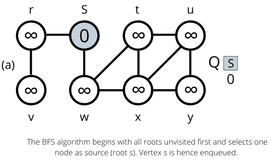
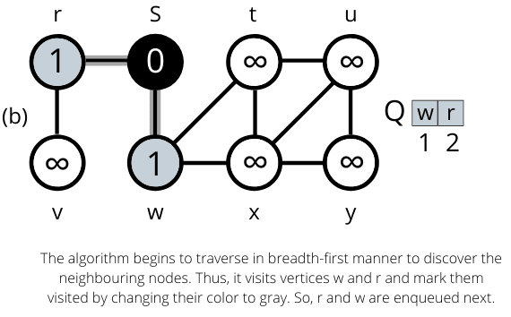
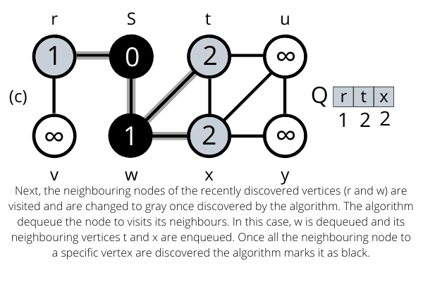
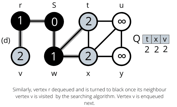
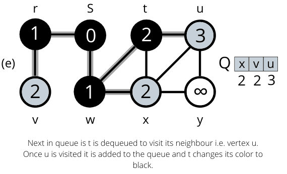
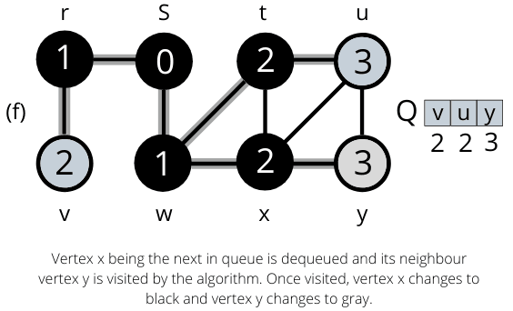
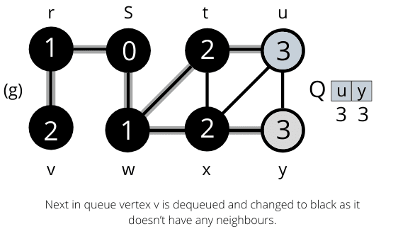
The operation of BFS on an undirected graph. Tree edges are shown as shaded as they are produced by BFS. The value of u.d appears within each vertex u. The queue Q is shown at the beginning of each iteration of the while loop. Vertex distances appear below vertices in the queue.

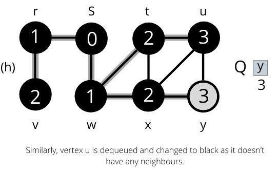
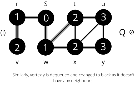Once all the nodes are visited the algorithm computes the shortest path between the root node s and its linking nodes. `

Complexity Analysis of BFS

Let us know consider analyzing the running time of the BFS algorithm on an input graph G= (V, E). After initialization, the breadth-first search never whitens a vertex and thus ensures that each vertex is enqueued and dequeued at most once. Time taken by each enqueue and dequeue operations is O(1), and so the total time devoted to queue operations is O(V). The algorithm scans the adjacency list of every vertex at most once and when the vertex is dequeued. The sum of the lengths of all the adjacency lists account to ?(E), the time spent to scan the adjacency lists is O(E). The overhead for initialization is calculated to be O(V), and thus the total running time complexity of the BFS algorithm is O (V + E).

So, the algorithm runs in linear time concerning the size of the adjacency list representation of graph G.

Suggested Course

Advanced Algorithms (Graph Algorithms) in Java

Why do we need a BFS Algorithm?

BFS algorithm offers several reasons to be used when searching for your data in any dataset. It provides us with considerable aspects to make itself consider as an efficient algorithm. Some of the popular aspects are:

• It is useful for analyzing the nodes in the graph and constructing the shortest path traversal.
• The algorithm traverses a given graph with minimum iterations.
• The architecture of the algorithm is robust.
• The result of the BFS algorithm provides us with the highest level of accuracy.
• The iterations of the algorithm are seamless, and so do not get caught up in infinite loop problems.

Rules of BFS Algorithm

Enlisted below are rules for using the BFS algorithm:

• It uses a queue data structure (FIFO)
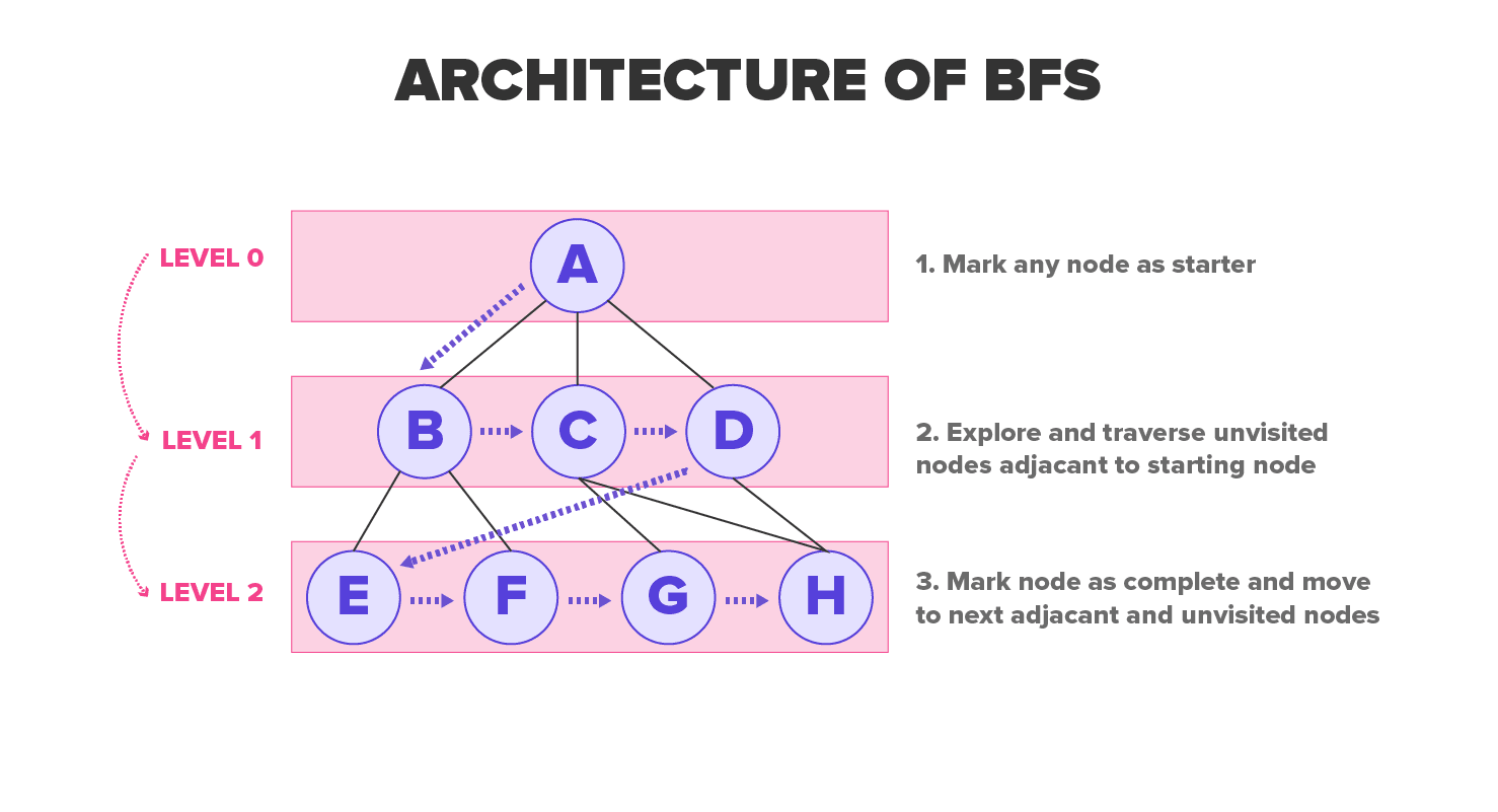
• Any node in the graph is marked as the root to begin traversal.
• It keeps dropping the node in the graph as it traverses through all nodes.
• The algorithm visits the adjacent unvisited nodes and keeps them inserting into the queue.
• In case no adjacent vertex is found, it removes the previous vertex from the queue.
• The BFS algorithm iterates until all the vertices are visited or traversed and marked as completed.
• The algorithm doesn't cause any loops during traversal of data from any node.

Breadth-First Search Algorithm Applications

Some of the real-life applications of the BFS algorithm implementation are listed below:

• Un-weighted Graphs: Shortest path in a graph and minimum spanning tree to visit all the vertices can be easily created using the BFS algorithm in the shortest time and high accuracy.
• P2P Networks: This algorithm is implemented to find the required data faster as it locates all nearest and neighboring nodes in a peer to peer network.
• Web Crawlers: The algorithm builds multiple levels of indexes for search engines and web crawlers. BFS implementation begins from the web page, which is the source and then visits all the links acting as nodes.
• Navigation Systems: Neighboring locations can be detected from the main or source location using the BFS algorithm.
• Network Broadcasting: A broadcasted packet is guided and tracked to search and reach all addressed nodes using the BFS algorithm.

Summary

That was the simple graph traversal algorithm, the breadth-first search algorithm. In summary, the graph traversal requires the algorithm to visit, check, and update, too(if needed), all the unvisited node in a tree-like structure. The BFS algorithm is known for analyzing the nodes in a graph and finding the shortest path of traversal. The BFS is an efficient algorithm with the complexity of O(V + E), and its graph traversal consists of a smaller number of iterations in the shortest possible time and doesn't get stuck in an infinite loop. The algorithm is used in multiple real-life applications such as web crawlers, P2P networks because of its robust nature. Have you noticed any application where you think the BFS algorithm could be at work behind it? Share with us in the comments below.

People are also reading:

• Best Data Science Tutorials
• Top 10 Python Data Science Libraries
• Top Data Science Interview Questions
• R for Data Science
• Data Science Applications
• Difference between Data Analyst vs Data Scientist
• 10 Best Data Science Books
• Python for Data Science
• Difference between Data Science vs Machine Learning
• Difference between Data Science vs Data Analytics
• Data Science Certification
• Data Science Degree
• Statistics for Data Science