Programmers use Big O notation for analyzing the time and space complexities of an algorithm. This notation measures the upper bound performance of any algorithm. To know everything about this notation, keep reading this Big O Cheat Sheet.
While creating code, what algorithm and data structure you choose matter a lot. Big O notation helps you compare the performance of various algorithms and find the right one for your type of code.
Today, in the modern world of complex applications and software, it is necessary to perform well in a different environment. For this, you need to optimize your code without any lag while executing the underlying code. Whenever you get the result of the Big O notation, you will be able to check if you have a lower running time than your competitors.
Thus, it has become necessary for programmers to check their code and analyze it thoroughly. This Big O Notation cheat sheet (time complexity cheat sheet or data structure cheat sheet) will help you understand various complexities.
Big O Cheat Sheet
This Big O cheat sheet is intended to provide you with the basic knowledge of the Big O notation. To begin with, we shall briefly discuss what exactly the Big O notation is. Further, we will look at various time and space charts and graphs for various algorithms.
For a deeper understanding of Big-O concepts for interview prep, I'd also recommend something like the Big-O Notation for Interviews course on Educative.
What is Big O Notation?
Big O Notation refers to a mathematical function applied in computer science to analyze an algorithm’s complexity. It defines the runtime required for executing an algorithm, but it won’t tell you how fast your algorithm’s runtime is. Instead, it will help you identify how your algorithm’s performance will change with the input size.
As per the formal definition, we can define O(g(n)) as a set of functions and a function f(n) as a member of that set only if this function satisfies the following condition:
0 ≤ f(n) ≤ cg(n)0 ≤ f(n) ≤ cg(n)
If an algorithm carries out a computation on each item within an array of size n, that algorithm runs in O(n) time and performs O(1) work for each item.
What is Space and Time Complexity?
The time complexity of an algorithm specifies the total time taken by an algorithm to execute as a function of the input’s length. In the same way, the space complexity of an algorithm specifies the total amount of space or memory taken by an algorithm to execute as a function of the input’s length.
Both the space and time complexities depend on various factors, such as underlying hardware, OS, CPU, processor, etc. However, when we analyze the performance of the algorithm, none of these factors are taken into consideration.
The following are some complexities:
- Constant: O(1)
- Linear time: O(n)
- Logarithmic time: O(n log n)
- Quadratic time: O(n^2)
- Exponential time: 2 ^{polyn}
- Factorial time: O(n!)
- Polynomial-time: 2^{O(log n)}
Recommended Course
Time and space complexity analysis (big-O notation)
What is the Big O chart?
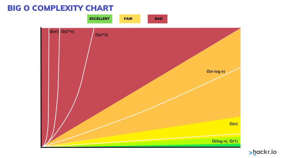
It is an asymptotic notation, allowing you to express the performance of algorithms or algorithm’s complexity based on the given input. Big O helps the programmers to understand the worst-case scenario and the execution time required or the memory used by an algorithm. Big O complexity can be understood with the following graph. This graph is also known as the Big O graph or Big O chart.

The following is a detailed explanation of different types of complexities with examples:
- Constant time: O(1)
An algorithm has a constant time with order O(1) when there is no dependency on the input size n. If there is no dependency, the runtime will remain the same throughout.
For example:
void printFirstElementOfArray(int arr[])

{

printf("First element of array = %d",arr[0]);

}
The above code will run in O(1) time concerning its input. Whether the above array has one item or 100 items, the function will require only one execution step. Thus, the function comes under constant time with order O (1).
- Linear time: O(n)
An algorithm will have a linear time complexity when the running time will increase linearly concerning the given input’s length. When the function checks all the values within input data, such type of function has Time complexity with order O(n).
For example:
void printAllElementOfArray(int arr[], int size)

{

for (int i = 0; i < size; i++)

{

printf("%d\n", arr[i]);

}

}
The function mentioned above will run in the O(n) time (or "linear time"), where n specifies the number of items within the array. Suppose the given array has ten items; the function will print ten times. If the number of items increases, the function will take that much time to print.
- Logarithm time: O(logn)
An algorithm will have a logarithmic time complexity when the size of the input data reduces in each step. It means that the number of operations is not the same as the input size. The number of operations will reduce with the increase in the input size.
Some examples of algorithms with Logarithmic time complexity are binary trees or binary search functions. It will include searching a given value in an array by splitting the array into two and starting searching in one split, ensuring that the operation is not done on every element of the data.
- Quadratic time: O(n^2)
void printAllElementOfArray(int arr[], int size)

{

for (int i = 0; i < size; i++)

{

printf("%d\n", arr[i]);

}

}
In the above example, we have nested two loops. If the array has n items, the outer loop will run the n times, and the inner loop will run the n times for each iteration of the outer loop, which will give total n2 prints. If the array has ten items, ten will print 100 times. Thus this function will run in the O(n^2) time.
- O(2^n)
int fibonacci(int num)

{

if (num <= 1) return num;

return fibonacci(num - 2) + fibonacci(num - 1);

}
The above example is the recursive calculation of Fibonacci numbers. O(2^n) specifies an algorithm where the growth gets double every time the input data set is added. The growth curve of an O(2n) function is exponential that starts as shallow and then rises meteorically.
- Drop the constants
Whenever you calculate the Big O complexity of any algorithm, you can throw out the constants.
For example:
void printAllItemsTwice(int arr[], int size)

{

for (int i = 0; i < size; i++)

{

printf("%d\n", arr[i]);

}

for (int i = 0; i < size; i++)

{

printf("%d\n", arr[i]);

}

}
This is O(2n), which we just call O(n).
void printHi100Times(int arr[], int size)

{

printf("First element of array = %d\n",arr[0]);

for (int i = 0; i < size/2; i++)

{

printf("%d\n", arr[i]);

}

for (int i = 0; i < 100; i++)

{

printf("Hi\n");

}

}
This is O(1 + n/2 + 100), which we just call O(n).
We only look for the big O notation when n gets arbitrarily large. As n gets big, adding 100 or dividing by two decreases significantly.
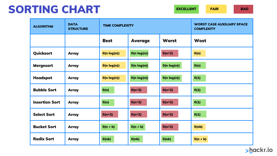
Algorithm Complexity Chart
Without getting the concept of algorithm complexity, you cannot understand the concept of the efficiency of algorithms and data structure.
Algorithm complexity is a measure that calculates the order of the count of operations carried out by an algorithm as a function of the size of the input data.
When we consider complexity, we speak of the order of operation count, not their exact count. In simpler words, complexity tells an approximation of the number of steps that execute an algorithm.
Big O Algorithm complexity is commonly represented with the O(f) notation, also referred to as asymptotic notation, where f is the function depending on the size of the input data. The asymptotic computational complexity O(f) measures the order of the consumed resources (CPU time, memory, etc.) by a specific algorithm expressed as the input data size function.
Complexity can be constant, logarithmic, linear, n*log(n), quadratic, cubic, exponential, etc.
|
Sorting Algorithms |
Space complexity |
Time complexity |
||
|
Worst case |
Best case |
Average case |
Worst case |
|
|
Insertion Sort |
O(1) |
O(n) |
O(n2) |
O(n2) |
|
Selection Sort |
O(1) |
O(n2) |
O(n2) |
O(n2) |
|
Smooth Sort |
O(1) |
O(n) |
O(n log n) |
O(n log n) |
|
Bubble Sort |
O(1) |
O(n) |
O(n2) |
O(n2) |
|
Shell Sort |
O(1) |
O(n) |
O(n log n2) |
O(n log n2) |
|
Mergesort |
O(n) |
O(n log n) |
O(n log n) |
O(n log n) |
|
Quicksort |
O(log n) |
O(n log n) |
O(n log n) |
O(n log n) |
|
Heapsort |
O(1) |
O(n log n) |
O(n log n) |
O(n log n) |
Typical Algorithm Complexities
The following table will explain different types of algorithm complexities:
|
Complexity |
Running Time |
Description |
|
constant |
O(1) |
It takes a constant number of steps to carry out a given operation (for example, 2, 4, 6, or another number), independent of the size of the input data. |
|
logarithmic |
O(log(N)) |
It takes the order of log(N) steps, with logarithm base 2, to carry out a given operation on N elements. For example, if N = 1,000,000, an algorithm with a complexity O(log(N)) would do about 20 steps. |
|
linear |
O(N) |
It takes nearly the same number of steps as the number of elements to operate on N elements. For example, if you have 1,000 elements, it will take about 1,000 steps. |
|
O(n*log(n)) |
It takes N*log(N) steps to carry out a given operation on N elements. For example, if you have 1,000 elements, it will take about 10,000 steps. |
|
|
quadratic |
O(n2) |
It takes the N2 number of steps, where the N specifies the input data size to carry out a given operation. For example, if N = 100, it will take about 10,000 steps. |
|
cubic |
O(n3) |
It takes the order of N3 steps, where N specifies the input data size to carry out an operation on N elements. For example, if N is 100 elements, it will take about 1,000,000 steps. |
Comparison Between Basic Data Structures
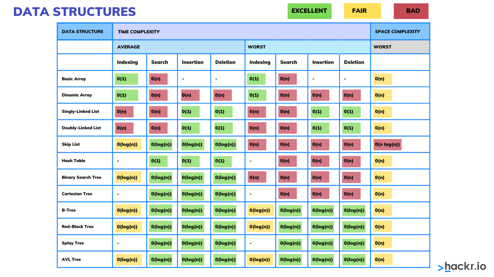
Now that you have understood the concept of the term algorithm complexity, we will look at the comparison between the basic data structures for estimating the complexity of each of them while performing the basic operations like addition, searching, deletion, and access by index (wherever applicable).
In such a way we could easily analyze the operations we want to perform and understand which structure would be appropriate. The complexities of carrying out the basic operations on the basic data structures can be seen in the following table.
|
Data structure |
Addition |
Search |
Deletion |
Access by index |
|
Array (T[]) |
O(N) |
O(N) |
O(N) |
O(1) |
|
Linked list (LinkedList<T>) |
O(1) |
O(N) |
O(N) |
O(N) |
|
Dynamic array (List<T>) |
O(1) |
O(N) |
O(N) |
O(1) |
|
Stack (Stack<T>) |
O(1) |
- |
O(1) |
- |
|
Queue (Queue<T>) |
O(1) |
- |
O(1) |
- |
|
Dictionary, implemented with a hash-table (Dictionary<K, T>) |
O(1) |
O(1) |
O(1) |
- |
|
Dictionary, implemented with a balanced search tree (SortedDictionary<K, T>) |
O(log(N)) |
O(log(N)) |
O(log(N)) |
- |
|
Set, implemented with a hash-table (HashSet<T>) |
O(1) |
O(1) |
O(1) |
- |
|
set, implemented with a balanced search tree (SortedSet<T>) |
O(log(N)) |
O(log(N)) |
O(log(N)) |
- |
Big O Notation Summary Table
|
Growth Rate |
Name |
Description |
|
1 |
Constant |
statement (one line of code) |
|
log(n) |
Logarithmic |
Divide in half (binary search) |
|
n |
Linear |
Loop |
|
n*log(n) |
Linearithmic |
Effective sorting algorithms |
|
n^2 |
Quadratic |
Double loop |
|
n^3 |
Cubic |
Triple loop |
|
2^n |
Exponential |
Exhaustive search |
Conclusion
Here we reach the end of the Big O cheat sheet. In this modern world surrounded by advanced technologies, creating complex software requires lengthy codes to process. But to improve the performance and reduce the time taken to carry out any task by the software, the code must be optimized. It is only possible by implementing a suitable array and data structure code.
The programmers need to analyze the complexity of the code by using different data of different sizes and determine what time it is taken to complete the task. If the time and space complexity are high, you can change your code and test again for its complexity. Big O notation is a function for analyzing the algorithm’s complexity. You can go through this Big O cheat sheet for a better understanding.
Interested in learning more about data structures, including more advanced data science projects? Try ProjectPro to implement big data where you work. They offer data science projects and schedule live, interactive sessions with experts. Or, when you want to upgrade your own skills, these DataCamp courses offer deep dives into many more topics.
FAQs
-
How do you calculate Big O easily?
To calculate Big O, you first need to consider how many operations are performed.
The following are simple steps:
- Split your algorithm into operations
- Calculate the Big O of each operation
- Add the Big O from each operation
- Strip out the constants
- Find the highest order term
For example: Adding two numbers
def add_nums(nums):

total = nums[0] + nums[1] # O(1) - Constant

 return total # O(1) - Constant

add_nums([1, 2, 3])
For total = nums[0] + nums[1], three operations are being performed, each having O(1) constant time complexity.
nums[0] – This is a lookup. O(1)
nums[1] – This is a lookup. O(1)
total = nums[0] + nums[1] – This is an assignment. O(1)
We then return the total, another O(1) operation.
-
What is Big O Notation for Dummies?
Big O notation, also referred to as the time complexity, implies the amount of time an algorithm takes to run. It indicates how long a specific algorithm runs as the data tends to grow.
-
What is the fastest O notation?
The fastest Big O notation is O(1) with constant time complexity.
-
What are the two rules of calculating Big-O?
The two most important rules are:
- Drop the constants
- Drop the Non-Dominant Terms
-
What is the big O of a while loop?
The Big O of a while loop depends on how you run it:
int i = 1; while ( i < n ) i ++; // O(n)
int i = 1; while ( i < n ) i *= 2; // O (log2( n) )
int i = 1; while ( i < n) { int j = 0; while ( j < n ) j ++; } // O( n * n )


